Use case 2: school class networks

This use case shows how a teacher uses MyNetworkmap to record, display and analyse friendship relations in several classes – with one project per class, a Kamada-Kawai layout and an interpretation of the computed centrality measures.

The example: Ms Lindner teaches at a comprehensive school and looks after three classes: 7a, 8b and 9c. She wants to know who is friends with whom in her classes, who is on the margin, and whether the classes differ across year groups.

A note on the data: the screenshots come from a real installation. The example data of the three classes was generated for this manual; all measures quoted are the values MyNetworkmap computed for that data.

---

Part 1: theoretical background

Sociometry: an old idea with new tools

The method of asking children who they are friends with and drawing a picture from it goes back to Jacob Levy Moreno, who developed the sociogram in the 1930s. Moreno worked with paper and ruler; the computation MyNetworkmap does in seconds then took days.

The core is unchanged: a nomination question (“whom do you like best in this class?”) produces directed relations from which the social structure of the group can be reconstructed.

What research says about school classes

Three findings are so well established that they belong in every analysis as an expectation:

Homophily. Children and adolescents befriend mostly those like themselves – most strongly by gender. Gender segregation is most pronounced at primary school age, still reaches high values in early secondary school, and dissolves over the course of adolescence. A survey across several year groups makes that trajectory immediately visible.

Reciprocity. Not every nomination is returned. Typical values are 30 to 50 per cent mutual nominations. The share of unreturned nominations is itself a finding: children who name many and are named by few often experience their position in the class differently from how it actually is.

Social position and well-being. The link between the number of incoming nominations and subjective well-being is one of the most stable findings in school research. Children without incoming nominations – isolates – consistently report lower well-being, more loneliness and less enjoyment of school.

What is particularly interesting today

The classical question “who is popular?” has largely been answered. More interesting at present – and well displayed with MyNetworkmap – are three follow-up questions:

Question	How you see it	Visualisation
Do friendships follow gender or origin?	Share of like nominations per property	Symbol colour and sector at the same time
Who mediates between separated groups?	High betweenness at moderate degree	Actor size by betweenness
Is position related to well-being?	In-degree against self-report	Actor size by well-being

The first question in particular can only be answered by showing two properties at once. That is exactly what MyNetworkmap's two independent channels on the symbol are for: the fill colour and the sector – the coloured ring.

Legal and ethical framework

Sociometric surveys with minors are delicate. Before the first question come:

• Consent from those with parental responsibility and assent from the children,
• approval by the school management and, depending on the state, the school authority,
• a clear statement of what the data will be used for.

The most important rule: individual-level results do not belong in the classroom. A sociogram with names projected on the wall is public exposure for the children at the margin. The map is a tool for the teacher and at most for one-to-one conversations – not for lessons.

Ask only about positive nominations, too. The classical rejection question (“whom would you not like to sit with?”) is unusual today for good reason: it directs the children's attention to exclusion.

---

Part 2: setting up the projects

Step 1: one project per class

Every class gets its own project:

• Klasse 7a – Schuljahr 2026/27
• Klasse 8b – Schuljahr 2026/27
• Klasse 9c – Schuljahr 2026/27

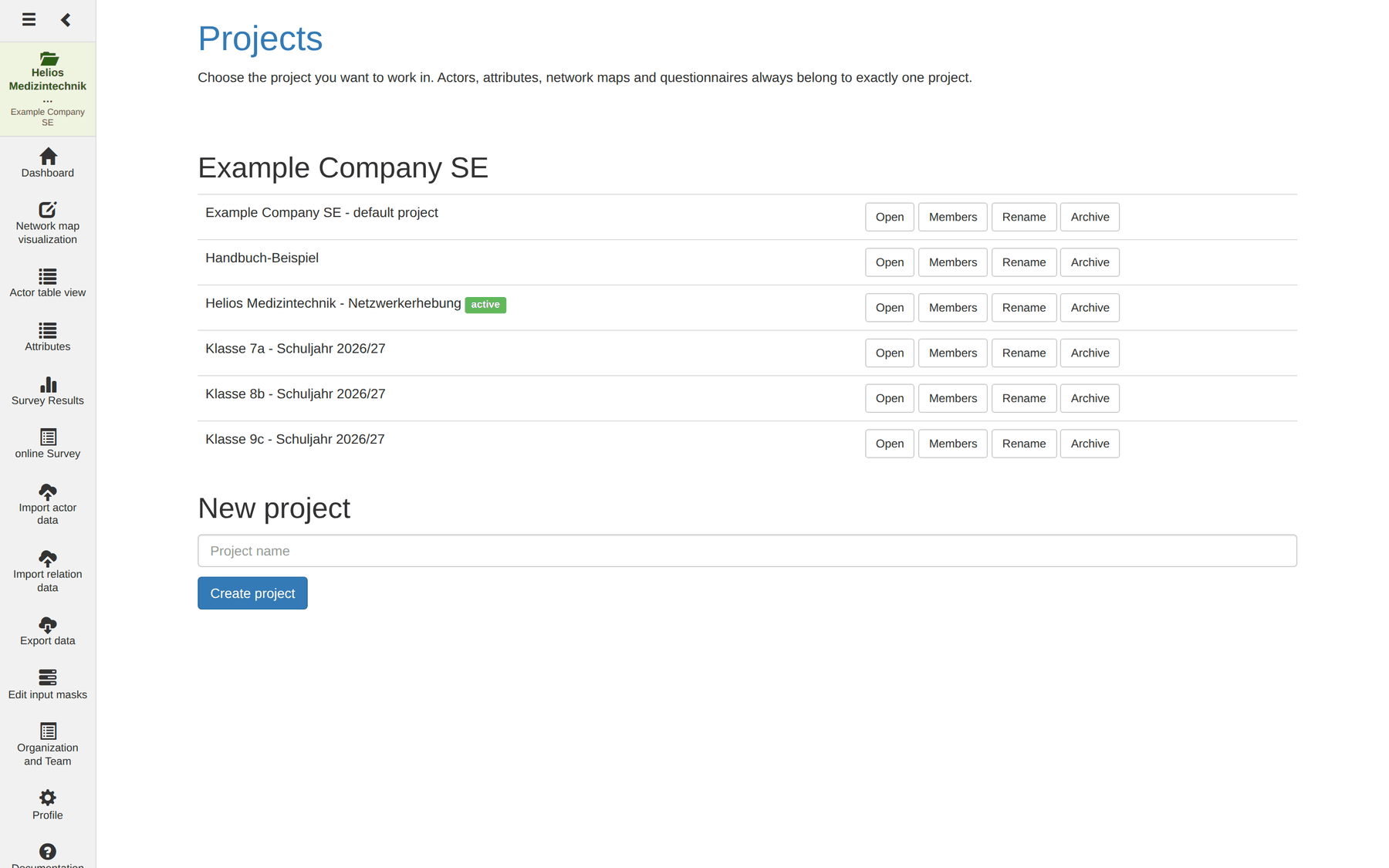
Why not all classes in one project? Because measures always refer to what lies on the map. With three classes on one map, density would measure the cohesion of three classes together – a meaningless number. Separate projects enforce the clean boundary and make the classes comparable with one another.

The school year is already in the project name: next year Klasse 8a – Schuljahr 2027/28 and so on are added, and the old data stays untouched.

Step 2: the attributes – and why they have to look like this

In each of the three projects you create the same attributes.

Actor attributes:

Attribute	Type	Values	What for
Name	free text	–	Present already
Geschlecht (gender)	predefined	weiblich, männlich, divers	Symbol colour
Alter (age)	free text	–	Description
Wohnort (district)	predefined	Kernstadt, Nordstadt, Seefeld, Umland	Actor sector
Wohlbefinden (well-being)	predefined	1, 2, 3, 4, 5	Actor size

Relation attribute:

Attribute	Type	Values
Freundschaft (friendship)	predefined	enge Freundschaft, Freundschaft, Bekanntschaft

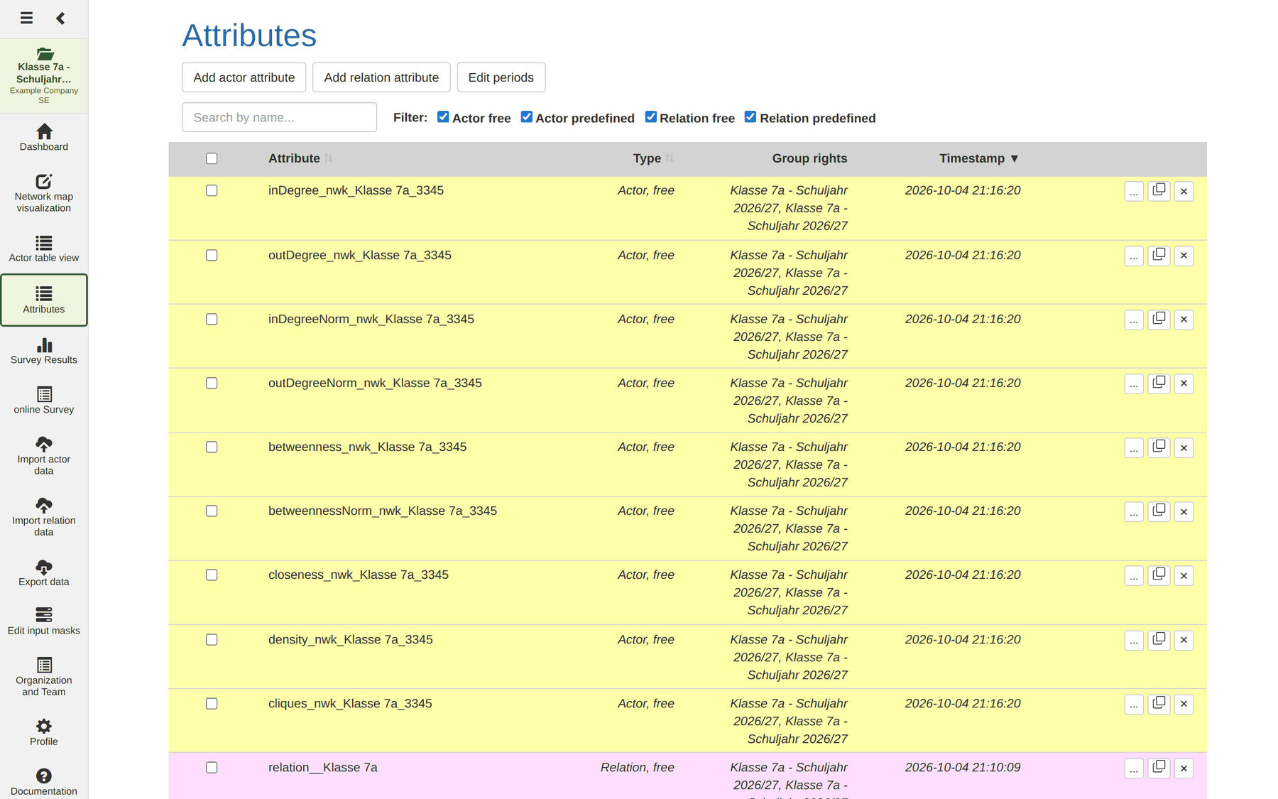
Caution – Wohnort must be predefined. As a free-text attribute it cannot be shown as a sector; the dialog then reports This attribute has no predefined attribute values. So create the four districts as a fixed value list instead of typing addresses freely. The same goes for Geschlecht and Wohlbefinden.

This decision cannot be changed afterwards – a free-text attribute never becomes a predefined one. Whoever makes it too late has to create a second attribute and transfer every value by hand.

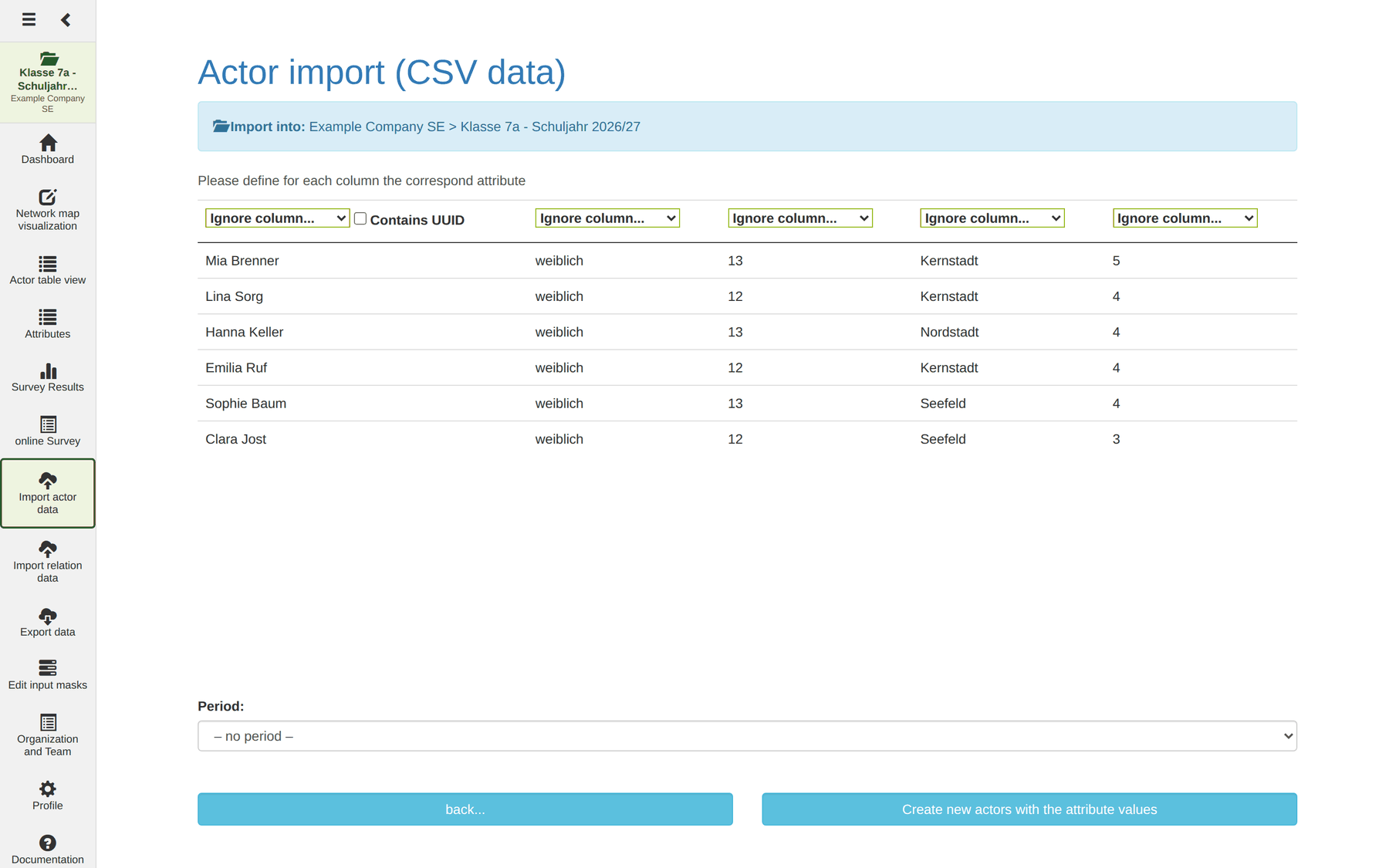
Step 3: import the class list

The CSV import is the quickest route. One row per child:

Name;Geschlecht;Alter;Wohnort;Wohlbefinden
Mia Brenner;weiblich;13;Kernstadt;5
Lina Sorg;weiblich;12;Kernstadt;4
Hanna Keller;weiblich;13;Nordstadt;4
…

Step 4: record the nominations

There are two routes for the survey itself:

• On paper, then through the relation import:

Von;Nach;Freundschaft Mia Brenner;Lina Sorg;Freundschaft Mia Brenner;Hanna Keller;Freundschaft …

• Online through a questionnaire with a predefined name list and individual links – exactly as described in use case 1. For school classes that has the advantage that children need not type anything and cannot misspell names.

---

Part 3: styling the network map

Step 5: create the map and enter the relations

1. Network map → Create new network map → name Klasse 7a, leave the option create necessary attributes automatically ticked.
2. + Relation → Freundschaft → directed (→) → Save.
3. + Relation → Freundschaft → reciprocal (↔) → Save.
4. Actors → add all actors.

Both relation entries are necessary. With only the directed entry, the map of 7a shows 58 lines instead of 79 – every mutual friendship is missing, that is, precisely the closest ones. The Relations counter in the Analysis section is the check: a conspicuously small number means the second entry is missing.

Step 6: the layout

Analysis → layout: Kamada Kawai, scaling 12, then start.

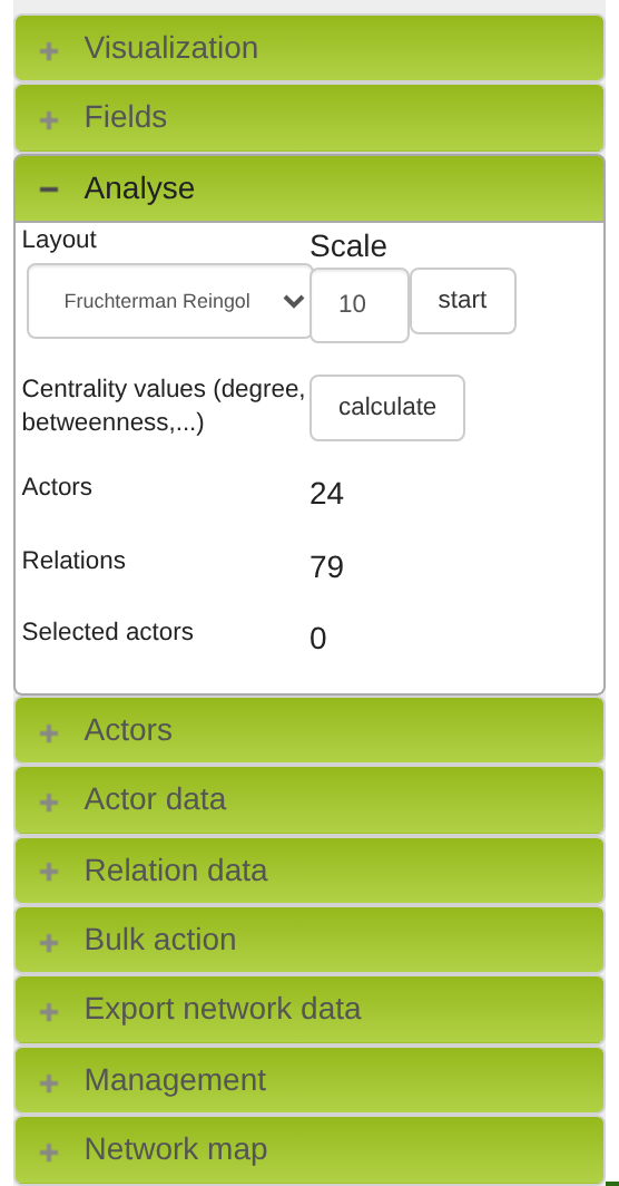
Why Kamada Kawai? The procedure tries to translate the graph-theoretic distance between any two nodes as faithfully as possible into a distance on screen. Whoever is far apart in the network is far apart in the picture. That produces spatially separated groups, with bridging people visibly in between – exactly what we want to see.

Fruchterman Reingold gives calmer pictures for large networks but separates groups less sharply. Circle arranges all nodes on a circle; that is useful for comparing the sheer number of edges but shows no group structure.

A layout is a display decision, not a result. What you interpret must be covered by the measures – not by the picture alone.

Step 7: the two visualisation channels

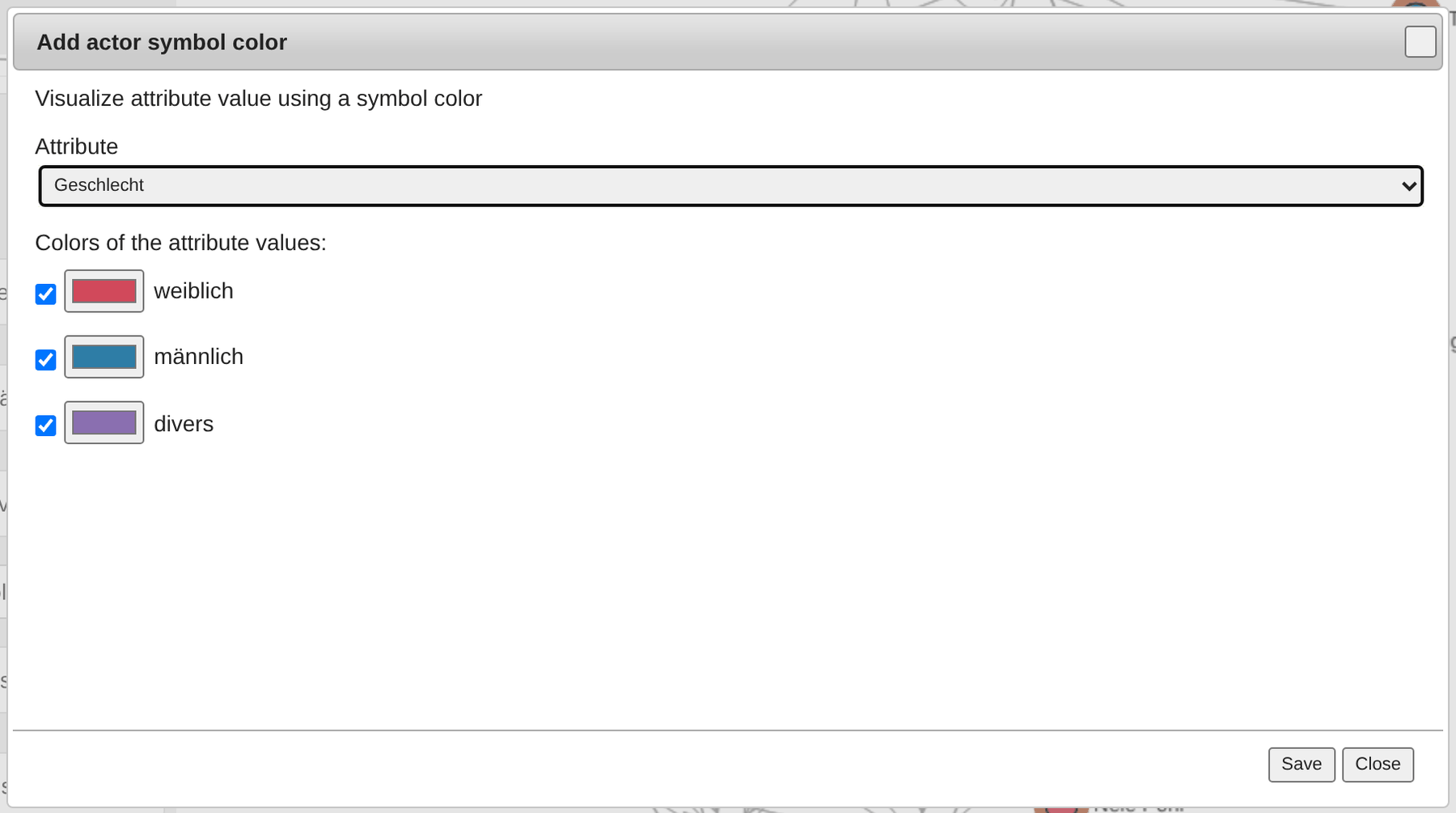
Actor symbol colour → Geschlecht:

Value	Colour
weiblich	red
männlich	blue
divers	violet

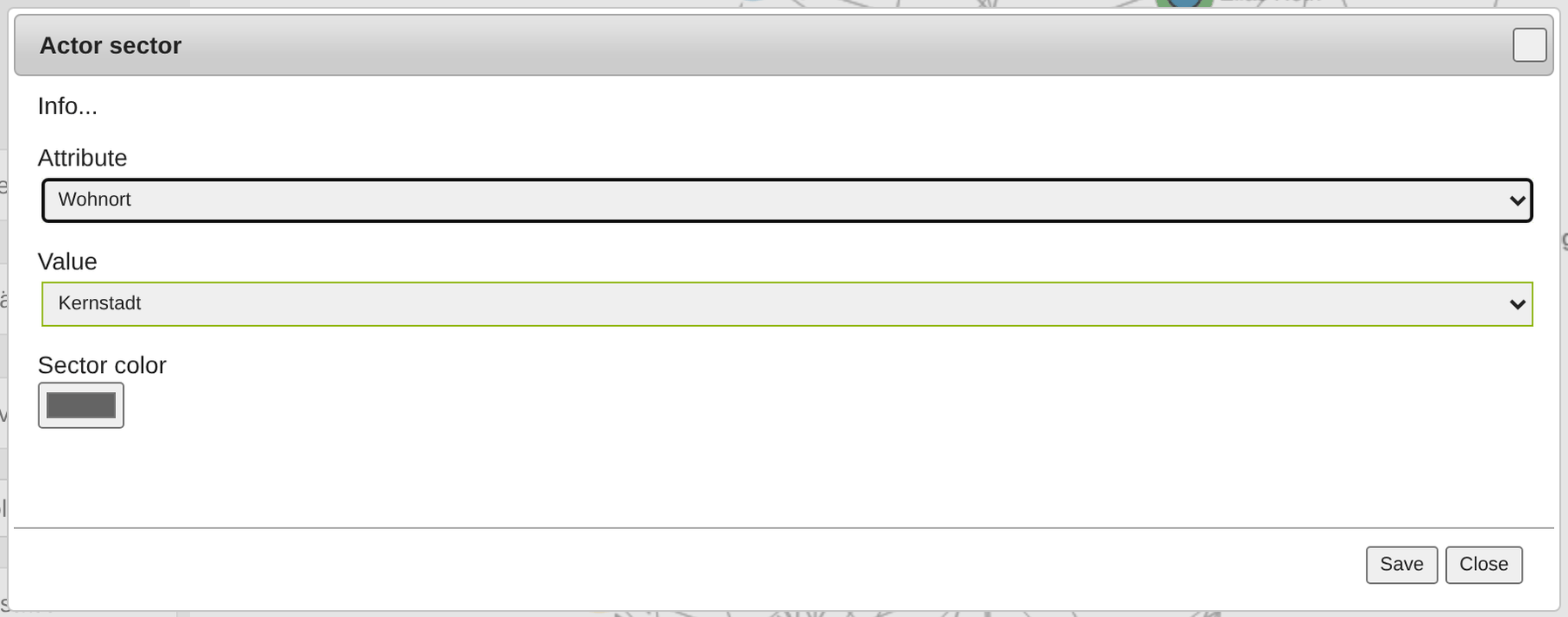
Actor sector → Wohnort: one colour per district – here yellow for Kernstadt, green for Nordstadt, blue for Seefeld, brown for Umland. The sector is created one value at a time: choose attribute, choose value, choose colour, Save – four times over.

The point of the double coding: the fill colour shows gender, the ring the district. If clusters form by fill colour, friendships follow gender; if they form by ring colour, they follow residence. The answer is in the picture before a single number has been computed.

Step 8: compute the measures

Analysis → centrality measures: compute now.

The values are stored as attributes (inDegree_nwk_Klasse 7a_… and so on) and can then be shown as columns in the actor table and sorted.

Tip: afterwards tie the symbol size to inDegree_nwk_… under Visualisation → actor size. The map then shows popularity as area – the picture becomes readable without further explanation.

---

Part 4: interpreting the results

Class 7a

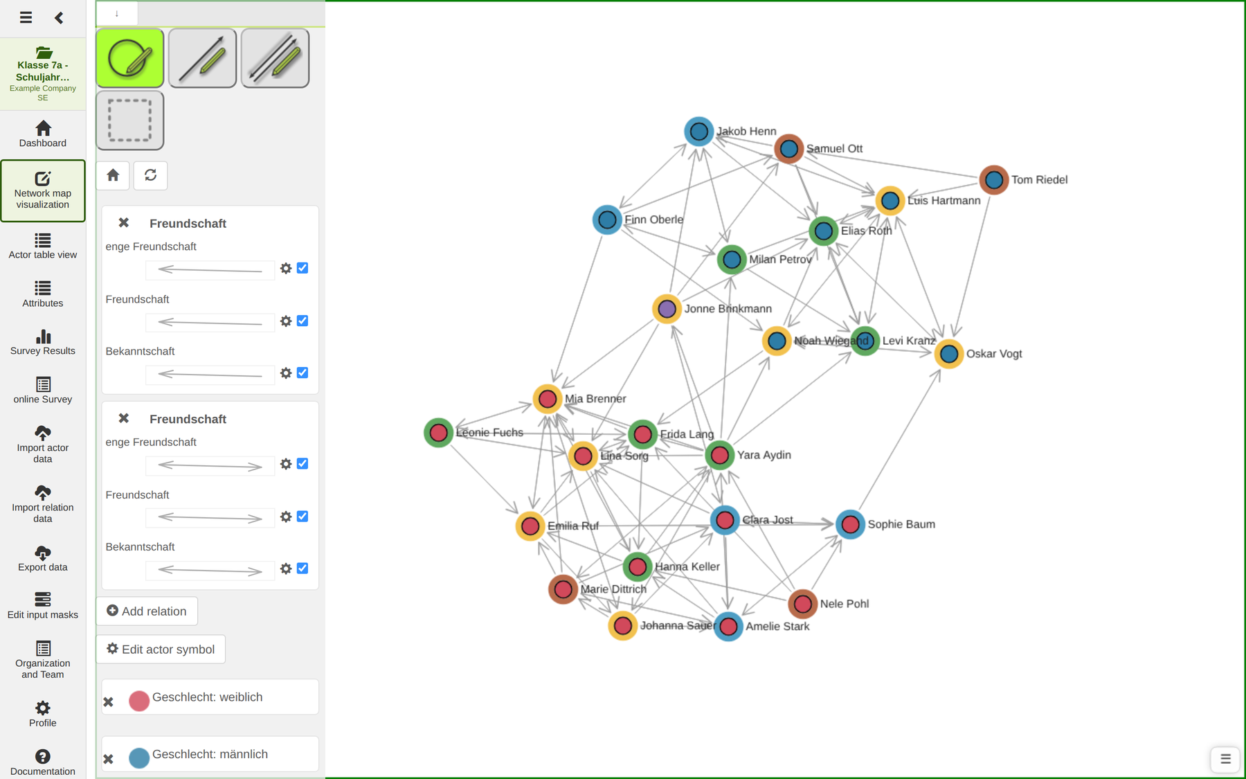
24 children, 100 nominations, 79 connected pairs, density 0.181.

At first glance the picture falls into two halves: a red block at the bottom left, a blue one at the top right. The ring colours, by contrast, are mixed across both halves. The figures confirm what you see:

Property	Share of like nominations
Gender	87 %
District	33 %

Friendships in 7a therefore follow gender almost entirely and residence hardly at all. With four districts, pure chance would give about 25 per cent like nominations – 33 per cent is barely above that.

Reciprocity: 42 % – a normal value.

The centrality measures:

Child	Gender	In-degree	Out-degree	Betweenness	Betw. norm.	Closeness
Yara Aydin	f	4	9	115.5	0.228	0.329
Mia Brenner	f	9	4	85.3	0.168	0.500
Frida Lang	f	6	4	84.5	0.167	0.489
Noah Wiegand	m	5	5	81.0	0.160	0.451
Luis Hartmann	m	8	5	44.5	0.088	0.426
Lina Sorg	f	8	3	22.3	0.044	0.469
…
Jonne Brinkmann	d	1	6	21.2	0.042	0.256
Nele Pohl	f	0	4	0.0	0.000	0.000
Tom Riedel	m	0	3	0.0	0.000	0.000

Finding 1: the most popular are not the most important. Mia Brenner (in-degree 9) and Luis Hartmann (8) are the stars of their respective halves. The highest betweenness, though, belongs to Yara Aydin with 115.5 – at an in-degree of only 4. She is the only child with an appreciable number of friendships into both halves of the class. She lies on almost 23 per cent of all shortest paths between any two children.

For classroom management she is the most interesting person: without Yara the class would fall into two barely connected groups. Her out-degree of 9 is striking too – she is the most active nominator in the class.

Finding 2: two children without a single nomination. Nele Pohl and Tom Riedel have an in-degree of 0. They name others themselves (4 and 3 respectively) but are named by nobody. Their closeness is 0 – in the directed network nobody reaches them.

Since all 24 children answered in this class, this is not non-response but a finding. Both live in the Umland – recognisable on the map by the brown ring – and both give the lowest Wohlbefinden value in the class, 2.

This is where network analysis ends and educational work begins. The map says that two children are on the outside and, with the district, offers one possible explanation: whoever lives out of town is not around in the afternoon. What follows from that – seating, group work, a conversation, an after-school club with transport – is for the teacher to decide, not the software.

Finding 3: a third kind of marginality. Jonne Brinkmann (divers) has an in-degree of 1 at an out-degree of 6. That is a different pattern from Nele and Tom: Jonne is not invisible but one-sidedly oriented – names many, is named by few. Such children often consider themselves well embedded; the discrepancy between self-image and nominations is the real finding.

Comparing the year groups

The real gain of the three separate projects shows in the comparison.

	7a	8b	9c
Children	24	26	22
Nominations	100	127	121
Density	0.181	0.195	0.262
Nominations of the same gender	87 %	70 %	55 %
Nominations in the same district	33 %	35 %	31 %
Reciprocity	42 %	28 %	35 %
Children without an incoming nomination	2	2	2

Finding 4: gender segregation dissolves. From 87 through 70 to 55 per cent – and that at practically unchanged district homophily around 33 per cent. This is exactly the trajectory research describes for adolescence, and it is directly visible on the three maps: in 7a red and blue nodes stand in two blocks, in 9c they are mixed.

That district homophily stays constant is the second half of the finding: residence never was the structuring factor and does not become one. That is precisely why the double coding pays off – without the sector you would not know what to contrast gender segregation against.

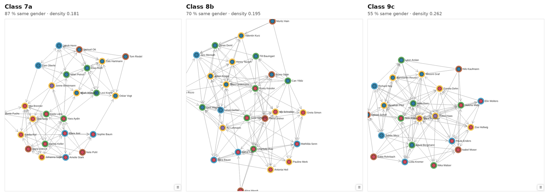
Finding 5: the classes get denser. Density rises from 0.181 to 0.262. In 9c practically every child knows and names a larger share of the class. That fits the dissolving gender boundary: when a dividing line falls away, more connections become possible – and they are used.

Finding 6: and yet somebody is left outside in every class. In all three classes there are exactly two children without an incoming nomination, and in all three cases they live in the Umland. A denser class is therefore not automatically a more inclusive one.

Finding 7: position and well-being go together.

Group	Average Wohlbefinden
Children with in-degree ≤ 1	2.0 – 2.3
Children with in-degree ≥ 6	3.8 – 4.1

The relationship appears with the same clarity in all three classes.

Careful with causality. The data shows an association, not a direction. Do children become unhappy because nobody names them? Or does nobody name them because they withdraw? Both are plausible, and both probably operate at once. A single survey cannot separate them – that would take a second wave with the same children.

A special case: Robin Haas in 9c

In 7a, Jonne Brinkmann (divers) is at the margin with an in-degree of 1. In 9c, Robin Haas (divers) has an in-degree of 10, an out-degree of 10, the highest betweenness in the class (63.8) and, with 13 cliques, membership in more subgroups than any other child.

Two individual cases are not a finding about year groups. But they are a good reason not to scan a class map only for isolates: the same combination of properties can lead to the margin in one class and to the centre in another.

The top of 9c

Mara Schuster reaches an in-degree of 16 – out of 21 possible. Her closeness is 0.808 and she appears in 12 cliques. Such a dominant position is unusual in a class of this size and deserves a second look: children like this carry a lot of social load, and the class becomes dependent on their mood.

---

Part 5: methodological notes

What the numbers cannot do

Limitation	Consequence
A snapshot	Friendships at this age change within weeks
One kind of relation	The survey says nothing about conflict or exclusion
Self-report	Children name whom they want to name
The class boundary	Friendships outside the class are invisible

The commonest mistake with school classes is to read the map as a diagnosis. It is a description of nominations at one point in time. A child without an incoming nomination is not “unpopular” – they were named by nobody on that day. The difference matters in a conversation with parents.

Repeat measurement

To find out whether a measure has worked, you need two points in time. Two routes are open:

• Periods in the same project – the children stay the same actors and the nominations are assigned to spans of time. The cleaner route for panels.
• A second project – easier to set up, but the actors are new and a comparison at person level takes handwork.

Checklist for a class survey

1. Consent obtained, school management informed.
2. One project per class, with the school year in the name.
3. Attributes created – Geschlecht, Wohnort, Wohlbefinden predefined.
4. Class list imported.
5. Positive nominations only.
6. The relation put on the map twice: directed and reciprocal.
7. Kamada-Kawai layout, colour and sector set.
8. Centrality measures computed – and recomputed after every change to the data.
9. Before passing anything on, checked: is there a name on it that should not be?