Network map

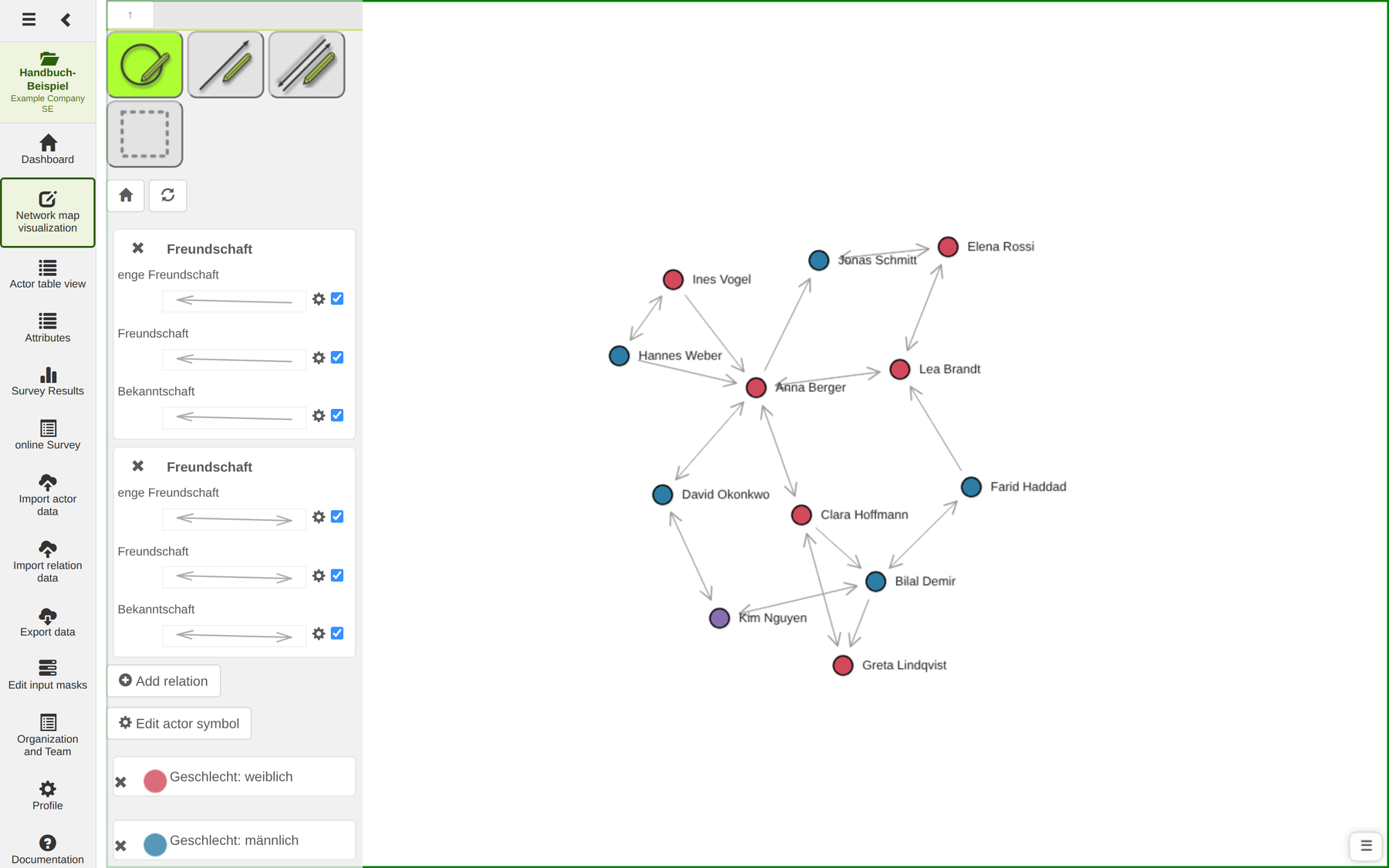
The network map is the heart of MyNetworkmap. Here data becomes a picture: actors appear as symbols, their relations as lines between them. You draw the network with the mouse, decide which properties become visible through colour, shape, size and sector, have a layout computed, derive measures and export the result.

A project can hold several network maps. All of them draw on the same stock of actors and attributes but show their own section with their own styling.

Note: the maps under Management are those of the active project.

Viewing, zooming and panning is open to every member – including the role Read only. Drawing, moving actors and styling need at least Survey, creating new attributes the role Editor.

Page layout

Area	Function
Toolbar (top left)	Choose the drawing mode, reset and refresh the view
Canvas	The map itself
Side menu (left)	Relations, styling, analysis, export, settings
Divider	Draggable: splits map and table
Actor table (bottom)	The same table as in the Actors module, linked to the map

The ↑ button above the side menu collapses it and gives the map more room.

Creating the first map

If a project has no map yet, the module opens the Create new network map dialog by itself. Otherwise you reach it through Management → Create new network map.

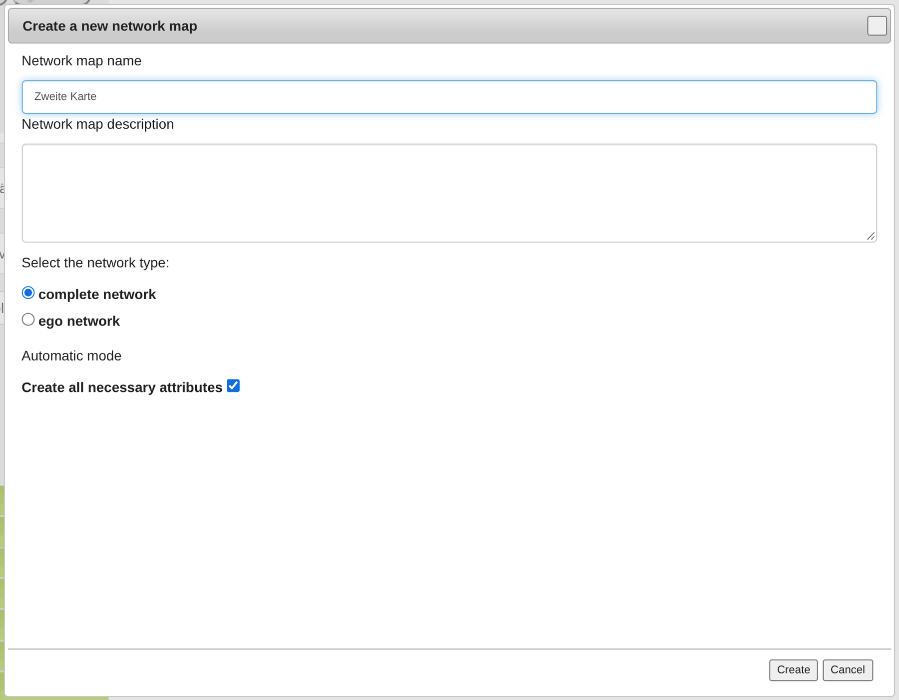
Field	Meaning
Network map name	Appears in the map list and in the names of the technical attributes
Network map description	Free text
complete network / ego network	Whole network or ego-centred network
create necessary attributes automatically	Creates the map's technical attributes

Caution – this option must stay ticked. “Create necessary attributes automatically” is not a convenience but a precondition. The map uses it to create three attributes:

Attribute	What for
nwk_<map name>	Remembers which actors lie on this map
nwk_x__<map name>	X position of each actor
nwk_y__<map name>	Y position of each actor

Without them the map cannot take a single actor: add all actors runs through and the map still stays empty. A relation attribute relation__<map name> is created as well, for relations drawn directly on this map.

After Create the map exists and is open – empty at first.

The toolbar

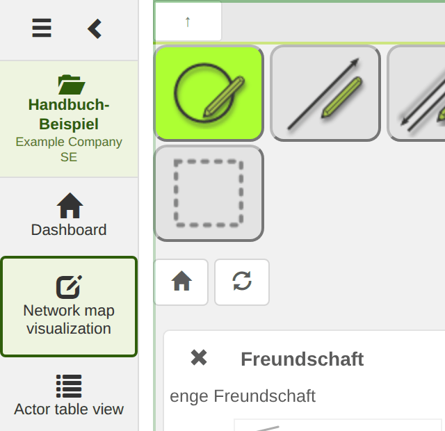
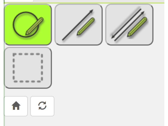
The top row selects the drawing mode; the active one is highlighted green.

Symbol	Mode	Meaning
Circle with pen	Draw actor	Create new actors on the map
Line with pen	Draw directed relation	A relation with one direction (→)
Double line with pen	Draw undirected relation	A relation both ways (↔)
Dashed rectangle	Select actors	Mark several actors with a rubber band

Below that:

• House – reset: resets zoom and viewport.
• Circular arrow – refresh: reloads the map, for instance after changes in the actor table.

Getting actors onto the map

There are three routes.

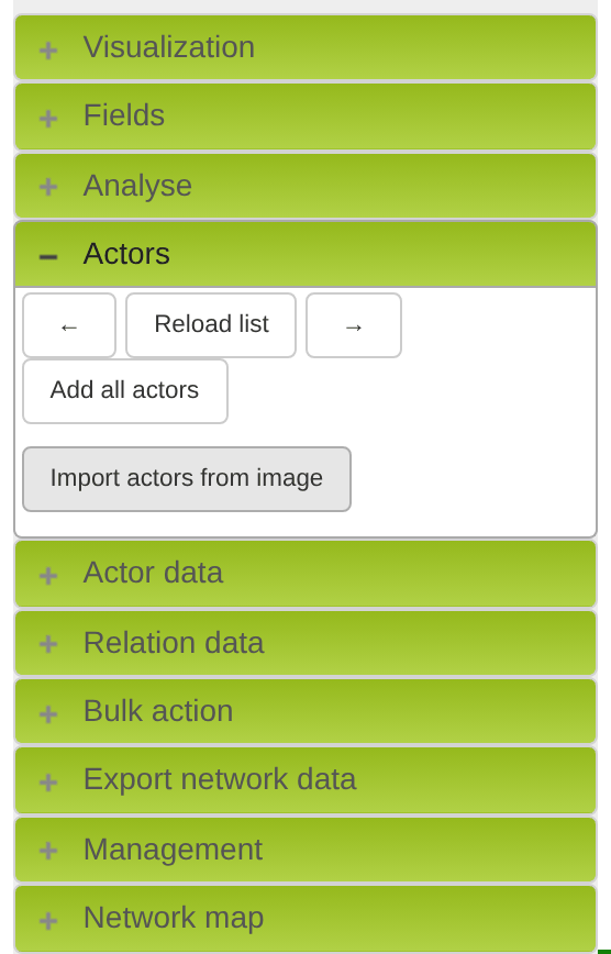
Fetch existing actors. In the side menu under Actors: Refresh list loads the actor list, the arrows ← and → page through it, add all actors puts every actor of the project on the map. This is the usual route after an import or a survey.

Draw new actors.

1. Select the mode Draw actor.
2. Click where you want it.
3. Click the context button (+) that appears.

Tip: after add all actors every node sits on top of the others in the middle of the map. That is normal – run a layout next.

Drop something onto it. The map accepts what you drag onto it from another window. What comes out of that depends on what you drag:

Dragged from	Result
A range of cells in Excel or LibreOffice Calc	Table import, see below
The actor list in the side menu	The existing actor lands where you dropped it
Any text	A new actor carrying that text as its name
An image on a web page	A new actor with that image

Where you let go is where the actor sits on the map.

Note: if what you dropped matches none of these, the map says so and creates nothing.

Importing a table by drag & drop

In Excel or LibreOffice Calc, select a range of cells including the header row and drag it onto the map. Every row becomes an actor, every column an attribute, and the header row supplies the attribute names. More than 500 rows or 50 columns is refused.

Before anything is created, a dialog asks for every column how it should be treated. Which options it offers depends on whether an actor attribute of that name already exists in the project:

State of the column	Options offered
The attribute does not exist yet	New categorical attribute · new free-text attribute · skip the column
The attribute exists as free text	Use the existing one · create a categorical one · create an additional free-text attribute · skip
The attribute exists as categorical, every value known	Use the existing one · skip
The attribute exists as categorical, with new values among them	Add the new values as further categories · create an entirely new categorical attribute · create an entirely new free-text attribute · skip

Categorical comes preselected as soon as a column holds fewer distinct values than rows – a sign that the values repeat and work as categories. Where every value differs, names for instance, the dialog suggests free text. What separates the two is described under attributes; colour, shape and sector on the map need categorical attributes.

When a column carries the same name as the label attribute of this map, the dialog says so – that column becomes the label of the new nodes.

The same dialog lets you pick a period for the new actors: an existing one, none, or a new one that you create right there with a name and an optional start and end date.

The new actors are staggered from the drop position: 50 points lower per actor, and after 500 points a new column starts 200 points further right. Empty rows are skipped.

What this route cannot do: it creates actors and their attributes, but no relations. Those come from the relation import, which expects a table with one row per relation.

Tip: this import is meant for the quick intermediate step – a list of names out of an e-mail, a list of participants out of a spreadsheet. For larger or recurring amounts of data the import module is the better route: it knows actor ids, it can update rather than only create, and it brings relations along.

Permission: like every import this route asks for the role Editor at least – it can create new attributes and categories and thereby changes the structure of the project. The other drag & drop forms above only create actors and are content with the role Survey.

Setting up relations

The top of the side menu lists the relations drawn on this map.

Each entry shows the relation attribute and, per attribute value, a row with a line preview and three controls:

Element	Function
✕	Remove the relation from this map
Gear	Edit the appearance (colour, width)
Checkbox	Show or hide the relation without removing it

+ Relation opens the Add relation dialog.

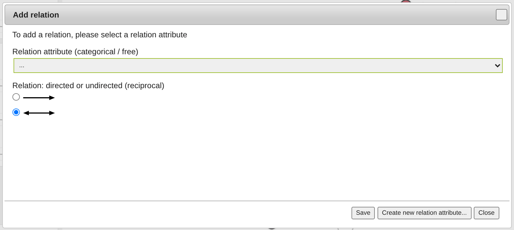
1. Choose the attribute under Relation attributes (categorical / free).
2. Set the direction under Relation: directed or undirected / reciprocal (→ or ↔).
3. Click Save.

If a suitable attribute is missing, create it right here with Create new relation attribute….

The most important point in this chapter

Add every relation attribute twice – once directed, once reciprocal.

The map draws one line per pair of actors. The rules are:

Entry on the map	What gets drawn
directed (→) only	only the pairs where the relation is one-sided
reciprocal (↔) only	all pairs, but without direction information
both	one-sided pairs as an arrow, mutual ones as a double arrow

Take class 7a from use case 2: 100 nominations among 24 children, of which 21 pairs are mutual and 58 one-sided.

• Directed only → 58 lines; every mutual friendship is missing.
• Reciprocal only → 79 lines; all there, but without direction.
• Both → 79 lines with the correct direction.

Forget the second entry and you see a network in which precisely the closest – because mutual – relations are absent.

Styling actors

Below the relation list are five buttons that make attribute values visible.

Button	Effect
Edit actor symbol	Show an attribute value through the symbol shape
Actor symbol colour	Show an attribute value through the symbol colour
Edit actor sector	Show an attribute value as a coloured ring on the symbol
Edit actor image	Link attribute values to images of your own
Actor filter	Show only actors that satisfy a condition

Actor symbol colour

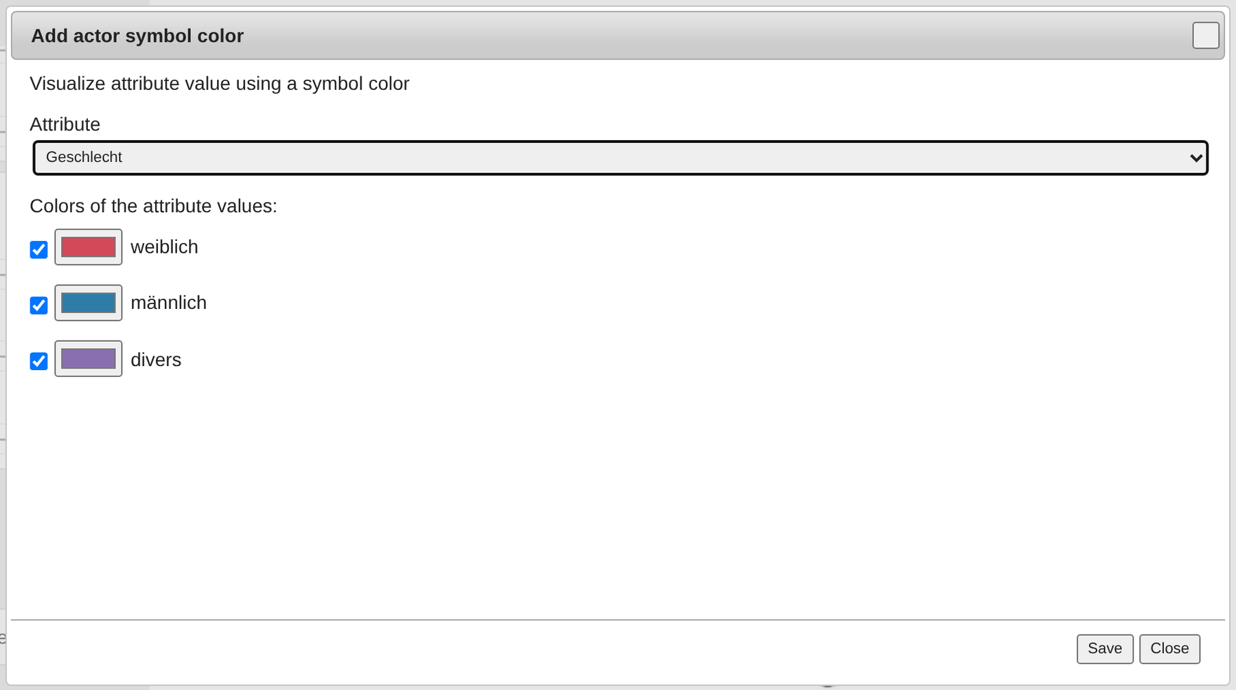
After selecting an attribute, all predefined values appear under Colours of the attribute values:. For each value you pick a colour and activate it with the checkbox. If the attribute has no predefined values, the dialog reports This attribute has no predefined attribute values.

Actor sector

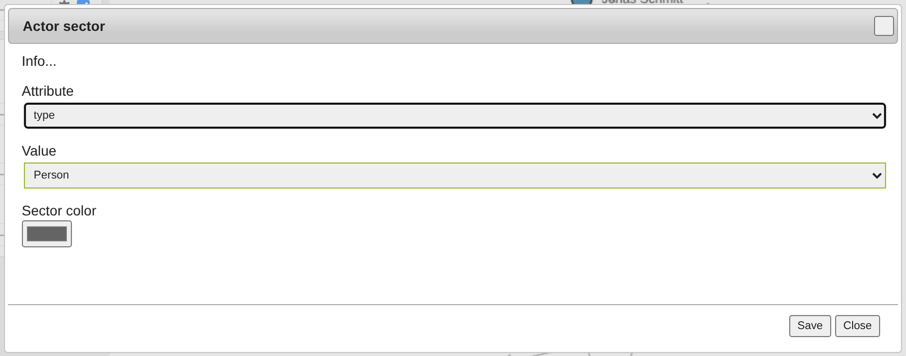
The sector is a coloured ring around the symbol. Unlike the symbol colour, you set it one value at a time:

1. Choose the attribute under Actor attributes.
2. Choose a value under Attribute value.
3. Choose a colour under Colour.
4. Save – and repeat for every further value.

Why two channels? Because they let you show two properties at once. In use case 2 the fill colour stands for gender and the ring for the district. At a glance you can see whether friendships follow gender or residence – a question you would otherwise have to compute.

Tip on colour choice: use clearly different colour families for fill and ring, and stay below five values per channel. More colours than that nobody can tell apart in print.

The side menu in detail

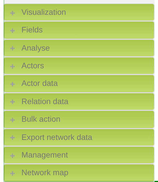
Below the styling buttons sits an accordion menu. Only one section is open at a time.

Visualisation

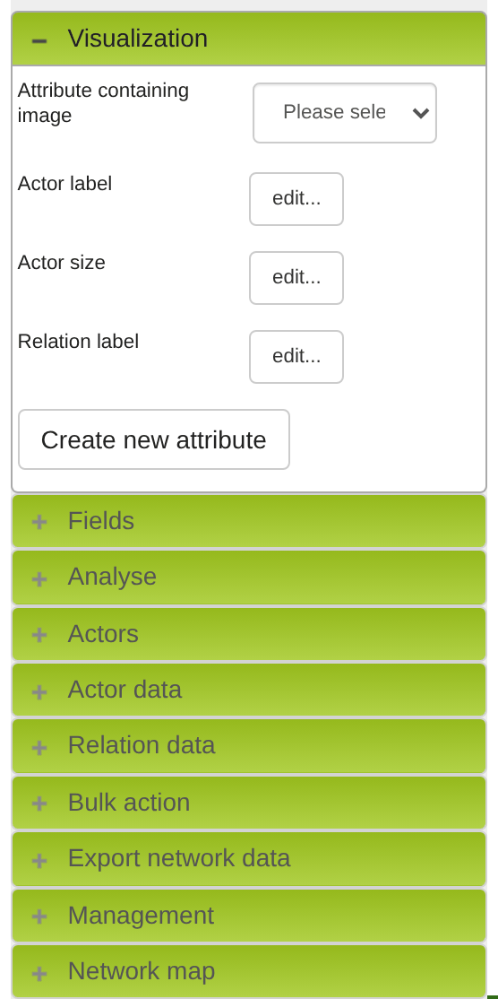
Setting	Meaning
Symbol	Base shape of the actor symbols
Attribute containing image	Which attribute supplies the actors' images
Actor label	Which attributes appear as the label, with font size and filter
Actor size	A fixed size or a size depending on an attribute value
Relation label	Labels on the lines and their font size

The edit… buttons open the respective dialog; Create new attribute leads into the Attributes module.

Actor size as a third channel: tie the size to a computed measure – say inDegree_nwk_… – and the map shows popularity directly as area. That is the fastest route from a list of numbers to a picture that non-specialists can read.

Fields

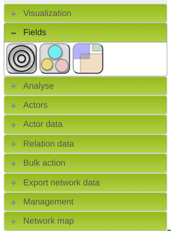
Fields – also called sensor fields – are areas on the map to which an attribute value is assigned. Place an actor inside one and the value is recorded for them. This supports proximity questions: the closer to the centre, the closer the relation.

The three buttons stand for circle fields (concentric circles), Venn circles and rectangle fields.

Analysis

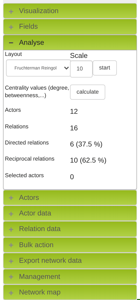
Layout arranges the actors automatically.

Algorithm	What it does	Suited to
Fruchterman Reingold	Force model: edges pull, nodes repel	General starting point, large networks
Kamada Kawai	Maps shortest-path distances as faithfully as possible	Medium-sized networks; shows groups and bridges most clearly
Circle	All nodes on a circle	Complete display without overlap; comparing edge density

Scaling determines how far the arrangement is pulled apart; start runs the computation.

Which layout? For groups of 15 to 50 actors, Kamada Kawai is usually the best choice: because it translates graph-theoretic distances into distances on screen, tightly connected subgroups end up near one another and bridging people visibly between them. Use case 2 builds on exactly that.

A layout is a display decision, not a result. The same data looks different with another algorithm. What you interpret has to be supported by the measures – not by the picture alone.

Centrality measures (degree, betweenness, …) computes the classical measures through compute now.

Important: the results are stored as new actor attributes, not merely displayed. For every measure an attribute is created following the pattern <measure>_nwk_<map name>_<map id>, for instance betweenness_nwk_Klasse 7a_3345. Created are: inDegree, outDegree, inDegreeNorm, outDegreeNorm, betweenness, betweennessNorm, closeness, density and cliques.

Afterwards these values behave like any other attribute: display them in the actor table, sort, filter, use them for the actor size and export them.

Caution: the computation refers to the actors and relations of this map – not to the whole project. If a relation entry is missing (the reciprocal one, say – see above), MyNetworkmap computes on an incomplete network and returns values that are too low. Check the Actors and Relations counters below before computing.

Recompute after every change to the data. The values are a snapshot; they do not update by themselves.

The counters

Below that you see what the map is made of. Every value refers to this map, not to the project, and is refreshed on every redraw.

Display	Meaning
Actors	Actors on the map
Relations	Connecting lines drawn
Directed relations	Of those, one-way – absolute and as a share
Reciprocal relations	Of those, mutual – absolute and as a share
Selected actors	Actors currently marked

Directed and reciprocal add up to 100 per cent because MyNetworkmap draws one line per connected pair of actors: the counter-direction of a mutual tie is skipped when drawing and therefore counted only once.

How the share is computed: dyad based, after Katz and Powell. Every connected pair of actors is classified once – as mutual (M) or asymmetric (A) – and the reciprocal share is M / (M + A). Unconnected pairs are left out; otherwise the value would fall simply because the network grew.

This is not the arc based reciprocity 2M / (2M + A) that some programs report, where a mutual tie counts as two edges. With 26 mutual and 16 asymmetric ties you see 61.9 per cent here; arc based it would be 76.5 per cent. Both are correct, they answer different questions: the share of pairs against the share of edges.

What to read from it: a high reciprocal share speaks for mutually confirmed relationships – for friendship questions in school classes it typically lies between 30 and 50 per cent. A strikingly low value often has a banal cause: only the directed relation type was put on the map. See The most important point in this chapter.

Actor data and relation data

These two sections show the data of the actor or relation you have selected, together with buttons to remove them.

Important – two different things: Remove actor from map takes the actor off this map only; they stay in the project. Delete actor removes them from the whole project for good, along with all their relations.

Bulk action

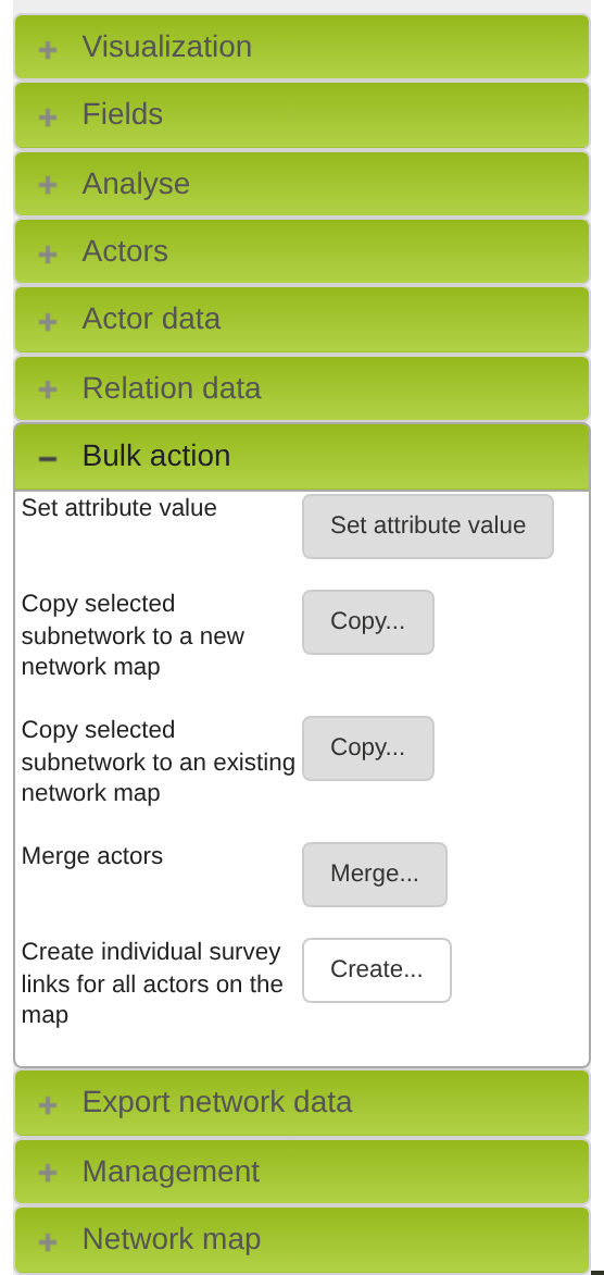
Bulk actions apply to all currently selected actors. Select them beforehand with a rubber band in the Select actors mode.

Action	Effect
Set attribute values	Give all selected actors the same value
Copy subnetwork to a new network map	Take the selection into a newly created map
Copy subnetwork to an existing network map	Insert the selection into an existing map
Merge actors	Merge several actors into one; the new one takes over all relations
Create an individual questionnaire link for every actor	One personal questionnaire link per actor

The last action is more powerful than its name suggests. It is the basis of every whole-network survey with named participants: everybody gets a personal link, the questionnaire therefore already knows who is answering, and the answers land on the right actor – without anybody typing their name and without duplicates. The full procedure is in use case 1.

The link is stored in the attribute questionnaireLink_<questionnaire name> and can be exported from there – for a mail merge, for instance.

Export

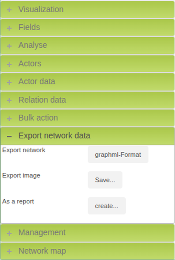
• Export network – graphml format: a GraphML file, readable in Gephi or yEd.
• Export image – save…: stores the map as a PNG file, in exactly the detail and zoom currently on screen.
• As a report – create…: produces a PDF report about the map, see below.

More extensive options are offered by the Export module.

The PDF report

The report records what the map shows at the moment it is created – not what the project holds altogether. Actors that are not on the map, filtered relations and deselected relation values stay out.

Section	Content
Header	Logo, name of the map, number of actors and relations, date of creation
The network map	The map as an image, with the legend as a table beneath it
Actors and attributes	One row per actor with their attribute values
Relations	Count per relation attribute, split into reciprocal and not reciprocal
Relations by attribute value	How often every single value of a relation attribute occurs
Network metrics	Density, indegree, outdegree, clustering coefficient, components, isolated actors
Glossary	What every metric means and how it is calculated

Which attributes the actor table holds follows from the map: the ones it visualises – label, symbol shape, symbol colour, size, sector – plus the columns set for the actor table beneath the map. To get an attribute into the report, show it as a column there.

The figures for reciprocal and not reciprocal relations are the same ones as in the Analysis section, counted the same way – once per connected pair of actors.

The report does not judge. It states figures and explains in the glossary how they come about. Whether a density of 12 per cent is high or low depends on the question being asked – that reading stays with you.

The language follows the interface. With the application set to German the report comes out in German, glossary included.

Tip: Set the map up the way you want to see it in the report before you click – the image takes over zoom, detail and filters unchanged. You need not open the legend for that: it is in the report as a table of its own anyway, and is deliberately left out of the image.

Management

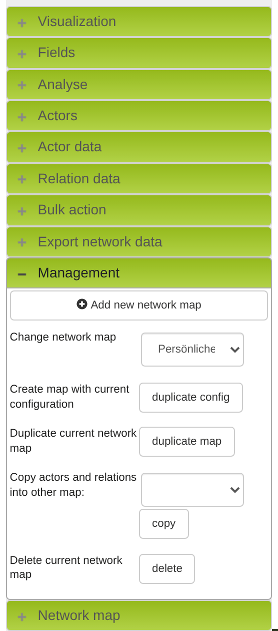
Row	Button	Effect
Add new network map	Add	Create an empty map
Change network map	dropdown	Switch between the project's maps
Create map with current configuration	duplicate config	A new map that takes over only the settings – without actors
Duplicate current network map	duplicate map	Full copy including actors and relations
Copy actors and relations into other map	copy	Transfer content into an existing map
Copy public network map to private map	copy from public	Take a publicly shared map over as your own
Delete current network map	delete	Remove the map

Tip: the distinction between duplicate config and duplicate map is meant for survey waves: take only the styling into an empty map when you need the same setup for a second point in time – and the whole map when you want to keep an intermediate state.

Network map

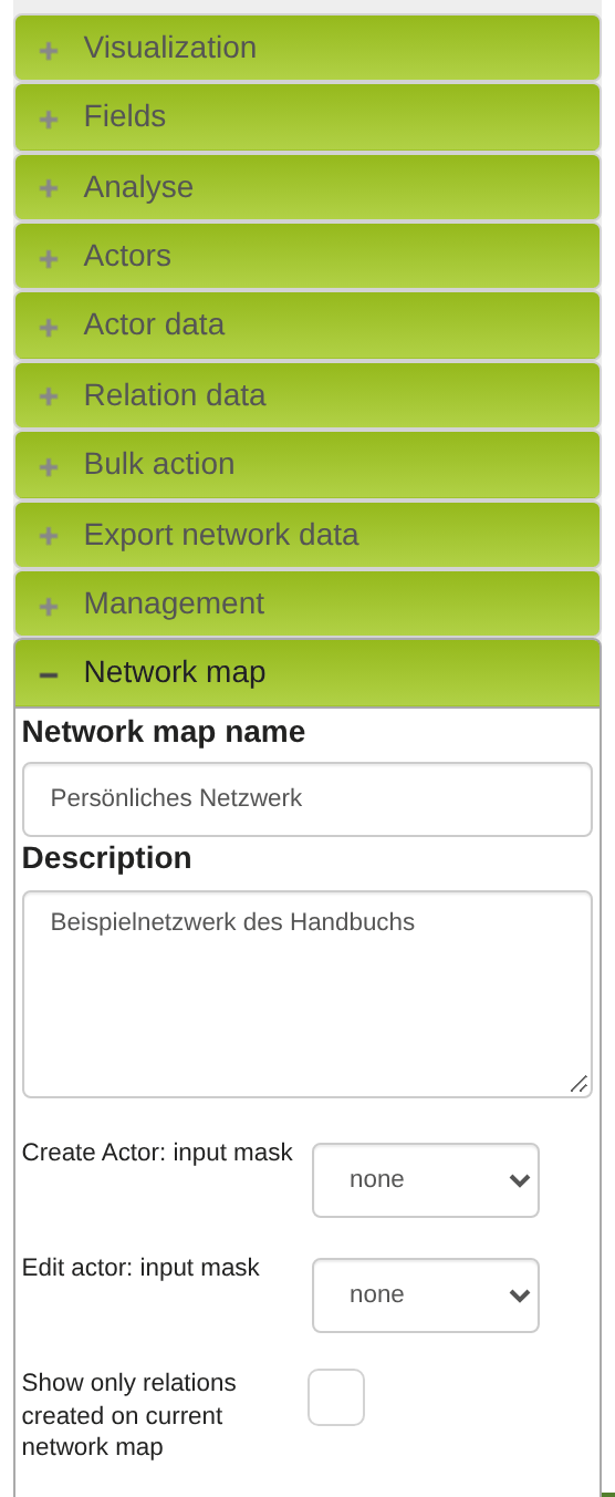
Setting	Meaning
Network map name	Name of the map
Description	Free text
Create Actor / Edit actor: input mask	Which input mask the respective dialog uses
X coordinate / Y coordinate	The attributes the positions are stored in – created by the map, shown here only
Show only relations created on current network map	Hides relations that arose elsewhere
activate team view	Working together as a team
Rotate network map / Rotate symbols	Rotates the display or the symbols
Ego settings with Set selected actor as ego	Ego-centred maps only: defines who the ego is
Filter attribute / Filter value	Restricts which actors the map accepts at all
Public (read only)	Releases the map for reading through a link

With Public (read only) active, the public link appears together with generate new link and Save to public map – the latter updates the published state.

Caution: anybody who knows the public link can view the map without signing in – labels included. With personal data that is rarely intended. Check the actor label before publishing and switch it to a pseudonym attribute if need be.

On rights to a map: the side menu has no section of its own for this. Who may read, edit or delete a map follows from the rights group of the project it belongs to and from your role in that project.

The actor table beneath the map

The lower part holds the same table as the Actors module – with its own column configuration per map. Map and table are linked both ways: clicking a node filters the table, clicking a row highlights the actor on the map. The divider can be dragged.

Building a map from scratch: the short version

1. Create the map – with create necessary attributes automatically ticked.
2. Add relation – the attribute once directed, once reciprocal.
3. Actors → add all actors.
4. Analysis → layout: Kamada Kawai, scaling 10–12, start.
5. Actor symbol colour on a predefined attribute.
6. Optionally actor sector for a second property.
7. Analysis → centrality measures: compute now.
8. Show the measures in the table, sort – and only then interpret.